class: center, middle, inverse, title-slide # MLCA Week 4: ## Imbalanced Classification ### Mike Mahoney ### 2021-09-22 --- class: center, middle # Classification, Continued --- class: middle Last week we started talking about classification using logistic regression, using a very simple model to predict employee attrition as a function of age. That simple model had ~89% overall accuracy -- not because it was highly predictive, but simply because ~89% of employees didn't quit, so our model could score high by assuming no one ever left. We're going to talk this week about ways to deal with that problem. --- class: middle Let's start by loading packages and recreating our dataframes: ```r library(modeldata) library(caret) library(pROC) library(dplyr) library(ggplot2) ``` <br /> First, we'll load the `attrition` data and clean it, using the same code as last week: ```r data(attrition) attrition_cleaned <- attrition |> mutate(across(where(is.factor), as.character)) |> mutate(Attrition = recode(Attrition, "Yes" = 1, "No" = 0)) ``` <br /> And then recreate our training and testing splits using the same code as before: ```r set.seed(123) row_idx <- sample(seq_len(nrow(attrition_cleaned)), nrow(attrition_cleaned)) training <- attrition_cleaned[row_idx < nrow(attrition_cleaned) * 0.8, ] testing <- attrition_cleaned[row_idx >= nrow(attrition_cleaned) * 0.8, ] ``` --- class: middle Last week we focused on an extremely simple model, with only Age as a predictor. <br /> This week, let's go ahead and use all the predictors in the data frame instead: ```r attrition_model <- glm(Attrition ~ ., training, family = "binomial") ``` <br /> And let's use a probability threshold of 0.5 to classify our predictions: ```r testing$prediction <- predict(attrition_model, testing, type = "response") testing$prediction <- round(testing$prediction) ``` --- We can use these predictions to calculate a new confusion matrix: ```r attrition_confusion <- confusionMatrix( factor(testing$prediction), factor(testing$Attrition), positive = "1" ) attrition_confusion ``` ``` ## Confusion Matrix and Statistics ## ## Reference ## Prediction 0 1 ## 0 250 18 ## 1 12 15 ## ## Accuracy : 0.8983 ## 95% CI : (0.858, 0.9303) ## No Information Rate : 0.8881 ## P-Value [Acc > NIR] : 0.3290 ## ## Kappa : 0.444 ## ## Mcnemar's Test P-Value : 0.3613 ## ## Sensitivity : 0.45455 ## Specificity : 0.95420 ## Pos Pred Value : 0.55556 ## Neg Pred Value : 0.93284 ## Prevalence : 0.11186 ## Detection Rate : 0.05085 ## Detection Prevalence : 0.09153 ## Balanced Accuracy : 0.70437 ## ## 'Positive' Class : 1 ## ``` --- As well as to take a look at our ROC curve and AUC: ```r attrition_roc <- roc( testing$Attrition, predict(attrition_model, testing, type = "response") ) ``` .center[ ```r plot(attrition_roc) ``` 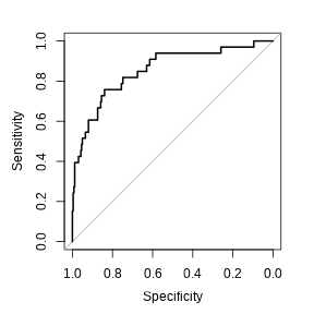<!-- --> ] ```r auc(attrition_roc) ``` ``` ## Area under the curve: 0.8547 ``` --- class: middle Even though our overall accuracy has barely changed -- 91% versus 89% -- we can tell from our sensitivity and AUC values that this model is much, much better at predicting which employees will quit. Meanwhile, our high specificity suggests we haven't gotten _that_ much worse at predicting which employees will stay. <br /> But we're still doing _much_ better at predicting employees who will stay than those who leave -- our sensitivity is about 45%, while our specificity is at 96%. <br /> Why does our new model, with so many more predictors to draw from, still mostly ignore "positive" cases? --- class: middle The answer is that there just aren't enough "positive" cases in our training data: ```r table(training$Attrition) ``` ``` ## ## 0 1 ## 971 204 ``` <br /> Our data set has almost 5 times more "No" values (0s) for attrition than "Yes"es (1s), so models which are super accurate on "No" and not very accurate on "Yes" can be just as accurate overall as a model trying its best on both classes. <br /> Our data has **imbalanced classes**, and this problem is an example of **imbalanced classification**. --- class: middle We have a handful of ways of dealing with imbalanced classes. One that we've already talked about is to change our probability threshold using our ROC curve. <br /> Another is to _weight_ our observations when we're fitting our model. We want our model to care about "Yes" just as much as "No", even though there are almost 5 times as many "No" values to predict. <br /> In this situation, we can provide weights to our model to signal that every "Yes" should be "worth" 5 times as much as each "No", so that in total both classes are "worth" the same amount to the model. --- class: middle To put this into practice, we'd first want to create a "weight" column in our training data set. We'll set the weights of "No" values to 1 and "Yes" to 5 to try and balance our classes: ```r training_weights <- ifelse(training$Attrition, 5, 1) training |> mutate(weight = training_weights) |> select(Age, Attrition, weight) |> head() ``` ``` ## Age Attrition weight ## 1 41 1 5 ## 2 49 0 1 ## 4 37 1 5 ## 5 33 0 1 ## 7 27 0 1 ## 8 32 0 1 ``` --- class: middle We then need to provide this new "weight" vector to the "weights" argument of `glm`: ```r weighted_model <- glm( Attrition ~ ., training, weights = training_weights, family = "binomial") ``` <br /> Then we make our predictions as we did originally: calculate the probability of each employee quitting, then use a probability threshold of 0.5 to classify employees into "Yes" and "No" groups: ```r testing$prediction <- predict(weighted_model, testing, type = "response") testing$prediction <- round(testing$prediction) ``` Let's take a look at our confusion matrix... --- ```r confusionMatrix(factor(testing$prediction), factor(testing$Attrition), positive = "1") ``` ``` ## Confusion Matrix and Statistics ## ## Reference ## Prediction 0 1 ## 0 206 8 ## 1 56 25 ## ## Accuracy : 0.7831 ## 95% CI : (0.7316, 0.8287) ## No Information Rate : 0.8881 ## P-Value [Acc > NIR] : 1 ## ## Kappa : 0.3325 ## ## Mcnemar's Test P-Value : 4.228e-09 ## ## Sensitivity : 0.75758 ## Specificity : 0.78626 ## Pos Pred Value : 0.30864 ## Neg Pred Value : 0.96262 ## Prevalence : 0.11186 ## Detection Rate : 0.08475 ## Detection Prevalence : 0.27458 ## Balanced Accuracy : 0.77192 ## ## 'Positive' Class : 1 ## ``` --- And take a look at our ROC curve and AUC: ```r weighted_roc <- roc( testing$Attrition, predict(weighted_model, testing, type = "response") ) ``` .center[ ```r plot(weighted_roc) ``` 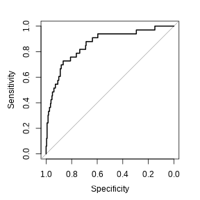<!-- --> ] ```r auc(weighted_roc) ``` ``` ## Area under the curve: 0.857 ``` --- class: middle So, to summarize, our weighted model has dramatically higher sensitivity than our original, at the cost of lower specificity and AUC. <br /> As we discussed last week, whether or not this is a _good_ thing strongly depends upon your goals for the model and what trade-offs you're willing to make. <br /> If you're happy to accept a more sensitive model at the cost of specificity -- to detect more positives overall even if it means you have more false positives -- then this is definitely an improvement. <br /> It might even make sense to weight the positives slightly more -- to intentionally imbalance your classes! --- A second way we might deal with imbalanced classes is to **resample** our data. To talk about resampling, it might make sense for us to talk first about sampling itself. Let's say we're interested in the heights of men across the USA. The heights for every man in the country might look something like this: ```r heights <- rnorm(1e5, mean = 68, sd = 4) qplot(heights) ``` <!-- --> --- But of course, it's rather expensive to measure every person in the country. Instead of doing that, most of the time we work with **samples** from our larger population. Ideally, our samples are chosen entirely at random, and each person is measured at most one time. If we only measure a few people, then our sample won't look anything like the population: ```r sampled_heights <- sample(heights, 10) qplot(sampled_heights) ``` <!-- --> --- But as we take more and more measurements, over time our measurements will start looking a lot more like the entire population: ```r sampled_heights <- sample(heights, 1e4) qplot(sampled_heights) ``` <!-- --> --- What if we took a sample that's larger than the population? Well, we'd need to break our rule that each person can only be measured once. We'd need to start taking measurements _with replacement_. We're still sampling at random, so any given person might be sampled once, more than once, or not at all. If we do that, our super-sized sample looks pretty much exactly like the population: ```r sampled_heights <- sample(heights, 1e6, replace = TRUE) qplot(sampled_heights) ``` <!-- --> --- class: middle This is the basic idea behind resampling methods. By taking samples with replacement from our sample, we can increase our effective sample size while still resembling the larger population, all without needing to go and collect new data. <br /> Of course, this method depends on our original sample being sufficiently representative of the population. If that wasn't true, though, you also wouldn't be able to fit good models _without_ resampling. <br /> But we can use this approach to increase the number of "Yes" observations we have in our data set, in order to balance our classes and make better predictions. --- class: middle To do that, we'd first split our training data into positive and negative pieces: ```r positive_training <- training[training$Attrition == 1, ] negative_training <- training[training$Attrition == 0, ] ``` Then we'd want to randomly select rows from our positive sample until we had the same number of positive observations as negatives. We can resample our positive sample to have five times the number of observations like this: ```r n_pos <- nrow(positive_training) resampled_positives <- sample(1:n_pos, size = 5 * n_pos, replace = TRUE) resampled_positives <- positive_training[resampled_positives, ] ``` --- Then we can combine our resampled positive dataframe with the original negative dataframe to get a new, evenly balanced data set: ```r resampled_training <- rbind( negative_training, resampled_positives ) ``` We can confirm that our classes are now balanced: ```r table(resampled_training$Attrition) ``` ``` ## ## 0 1 ## 971 1020 ``` <br /> If anything, we've actually added slightly too many "yes" cases to this data set! Now let's go ahead and fit a new model on the resampled data: ```r resampled_model <- glm( Attrition ~ ., resampled_training, family = "binomial") ``` --- class: middle Then we make our predictions as we did originally: calculate the probability of each employee quitting, then use a probability threshold of 0.5 to classify employees into "Yes" and "No" groups: ```r testing$prediction <- predict(resampled_model, testing, type = "response") testing$prediction <- round(testing$prediction) ``` <br /> Let's take a look at our confusion matrix... --- ```r confusionMatrix(factor(testing$prediction), factor(testing$Attrition), positive = "1") ``` ``` ## Confusion Matrix and Statistics ## ## Reference ## Prediction 0 1 ## 0 202 8 ## 1 60 25 ## ## Accuracy : 0.7695 ## 95% CI : (0.7172, 0.8163) ## No Information Rate : 0.8881 ## P-Value [Acc > NIR] : 1 ## ## Kappa : 0.313 ## ## Mcnemar's Test P-Value : 6.224e-10 ## ## Sensitivity : 0.75758 ## Specificity : 0.77099 ## Pos Pred Value : 0.29412 ## Neg Pred Value : 0.96190 ## Prevalence : 0.11186 ## Detection Rate : 0.08475 ## Detection Prevalence : 0.28814 ## Balanced Accuracy : 0.76428 ## ## 'Positive' Class : 1 ## ``` --- And take a look at our ROC curve and AUC: ```r resampled_roc <- roc( testing$Attrition, predict(resampled_model, testing, type = "response") ) ``` .center[ ```r plot(resampled_roc) ``` <!-- --> ] ```r auc(resampled_roc) ``` ``` ## Area under the curve: 0.8498 ``` --- class: middle Overall, this model is pretty similar in accuracy and AUC to the weighted version. That's not just coincidence; both of these methods were aiming at effectively increasing the importance of "Yes" values to the model by 500%, so it makes sense for two methods with the same goals to have similar outcomes. When you're able to specify weights, that's often a better way to adjust for imbalanced classes than resampling; it makes your intent more obvious and is computationally more efficient. But often, model implementations won't provide obvious ways to weight your classes, requiring you to try resampling instead. --- Note also these methods produce slightly different probabilities: <!-- --> <!-- --> <!-- --> --- class: middle These approaches can be used even with more complex models to try and deal with imbalanced classes. <br /> While new methods are being proposed every day -- imbalanced classification problems are one of the most fundamental unsolved problems in prediction -- setting thresholds based on ROC curves, weighting your classes, and resampling your data will be generally applicable to any real-world classification problem you have to work with. --- class: middle One final note: I want to highlight that both weighting and resampling used the class abundances from the _training set_. <br /> You should not be setting weights based on the prevalence of classes in the test set; as we mentioned week 2, the test data should be completely unknown to both the model and the modeler. <br /> That means you shouldn't even _know_ what the class abundances are in the test set, if you can avoid it. <br /> That's it for this week. Next week we leave the world of traditional statistics and start in with our first pure prediction algorithm: the decision tree.